7.2. Lesson: Analiza Vectorială¶

7.2.1. Procesul GIS¶

Before we start, it would be useful to give a brief overview of a process that can be used to solve any GIS problem. The way to go about it is:

1. Definirea Problemei

2. Obținerea Datelor

3. Analiza Problemei

4. Prezentarea Rezultatelor

7.2.2. Problema¶

Let’s start off the process by deciding on a problem to solve. For example, you are an estate agent and you are looking for a residential property in Swellendam for clients who have the following criteria:

1. Să fie situată în Swellendam.

2. Trebuie să fie situată la o distanță de conducere rezonabilă, față de o școală (de exemplu, 1 km).

3. Trebuie să aibăo dimensiune de peste 100m pătrați.

4. Să fie situată sub 50m față de un drum principal.

5. Să fie situată la maximum 500m față de un restaurant.

7.2.3. Datele¶

Pentru a răspunde la aceste întrebări, vom avea nevoie de următoarele date:

1. Proprietățile rezidențiale (clădirile) din zonă.

2. Drumurile din jurul și din cadrul orașului.

3. Amplasarea școlilor și a restaurantelor.

4. Dimensiunea clădirilor.

All of this data is available through OSM and you should find that the dataset you have been using throughout this manual can also be used for this lesson. However, in order to ensure we have the complete data, we will re-download the data from OSM using QGIS’ built-in OSM download tool.

7.2.4. Follow Along: Startarea unui Proiect¶

• Deschideți un nou proiect QGIS

• Use the OpenStreetMap data download tool found in the Vector -> OpenStreetMap menu to download the data for your chosen region.

• Salvați rezultatul ca osm_data.osm, în folderul exercise_data.

• Note that the osm format is a type of vector data. Add this data as a vector layer as usually Layer -> Add vector layer..., browse to the new osm_data.osm file you just downloaded. You may need to select Show All Files as the file format.

• Selectați osm_data.osm, apoi faceți clic pe Open

• În caseta de dialog care se deschide, selectați toate straturile, cu excepția straturilor other_relations și multilinestrings:

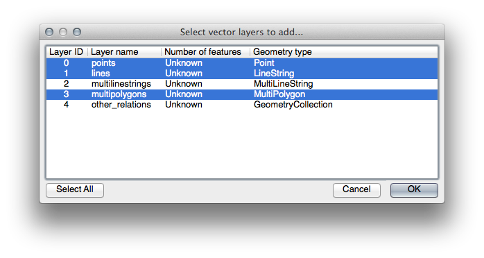
Acest lucru va importa datele OSM în hartă ca și straturi separate.

The data you just downloaded from OSM is in a geographic coordinate system, WGS84, which uses latitude and longitude coordinates, as you know from the previous lesson. You also learnt that to calculate distances in meters, we need to work with a projected coordinate system. Start by setting your project’s coordinate system to a suitable CRS for your data, in the case of Swellendam, WGS 84 / UTM zone 34S:

• Deschideți dialogul Proprietățile Proiectului, selectați CRS și filtrați lista pentru a găsi WGS 84 / UTM zone 34S.

• Clic pe OK

We now need to extract the information we need from the OSM dataset. We need to end up with layers representing all the houses, schools, restaurants and roads in the region. That information is inside the multipolygons layer and can be extracted using the information in its Attribute Table. We’ll start with the schools layer:

• Faceți clic-dreapta pe stratul multipolygons din Lista straturilor dvs., apoi deschideți dialogul Proprietăților Stratului.

• Mergeți la meniul General.

• În Subsetul Entităților faceți clic pe butonul [Query Builder] deschide dialogul Query builder.

• În lista Cămpurilor din partea stângă a acestui dialog, derulați până când veți vedea câmpul amenity.

• Faceți clic pe el o dată.

• Faceți clic pe butonul All de sub lista Valori:

Acum, trebuie să indicați aplicației QGIS să arate doar poligoanele în care valoarea amenity este egală cu school.

• Dublu-clic pe cuvântul amenity din lista Câmpurilor.

• Priviți ce se întâmplă în câmpul ExpresiIor de filtrare specifice furnizorului de mai jos:

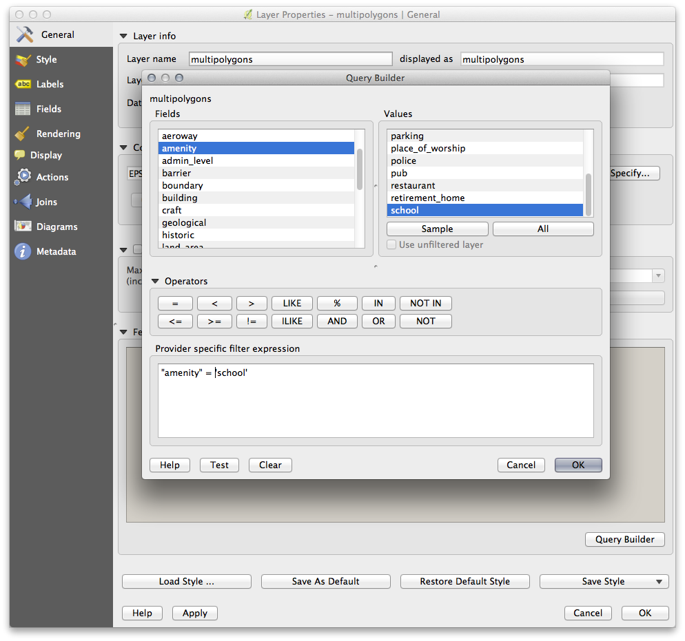
A apărut cuvântul "amenity". Pentru a construi restul interogării:

• Faceți clic pe butonul = (de sub lista Operatorilor).

• Dublu-clic pe valoarea school din lista Valorilor.

• Clic pe OK, de două ori.

This will filter OSM’s multipolygons layer to only show the schools in your region. You can now either:

• Rename the filtered OSM layer to schools and re-import the multipolygons layer from osm_data.osm, OR
• Duplicate the filtered layer, rename the copy, clear the Query Builder and create your new query in the Query Builder.

7.2.5. Try Yourself Extrageți Straturile Cerute din OSM¶

Using the above technique, use the Query Builder tool to extract the remaining data from OSM to create the following layers:

• roads (din stratul OSM lines)

• restaurants (din stratul OSM multipolygons)

• houses (din stratul OSM multipolygons)

Ați putea re-utiliza stratul roads.shp pe care le-ați creat în lecțiile anterioare.

Verificați-vă rezultatele

• Save your map under exercise_data, as analysis.qgs (this map will be used in future modules).
• In your operating system’s file manager, create a new folder under exercise_data and call it residential_development. This is where you’ll save the datasets that will be the results of the analysis functions.

7.2.6. Try Yourself Găsiți drumurile importante¶

Some of the roads in OSM’s dataset are listed as unclassified, tracks, path and footway. We want to exclude these from our roads dataset.

• Deschideți Constructorul de Interogări pentru stratul roads, clic pe Clear și construiți următoarea interogare:

  "highway"  != 'NULL' AND "highway" != 'unclassified' AND "highway" != 'track' AND "highway" != 'path' AND "highway" != 'footway'

You can either use the approach above, where you double-clicked values and clicked buttons, or you can copy and paste the command above.

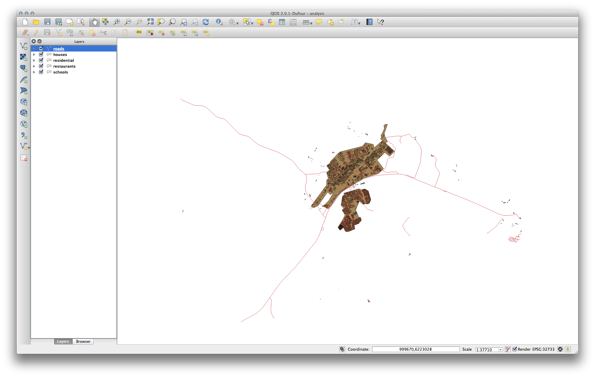
Acest lucru ar trebui să reducă imediat numărul de drumuri de pe hartă:

7.2.7. Try Yourself Convertiți CRS-ul Straturilor¶

Because we are going to be measuring distances within our layers, we need to change the layers’ CRS. To do this, we need to select each layer in turn, save the layer to a new shapefile with our new projection, then import that new layer into our map.

• Faceți clic-dreapta pe stratul roads din panoul Layers.

• Clic pe Save as...

• In the Save Vector As dialog, choose the following settings and click Ok (making sure you select Add saved file to map):

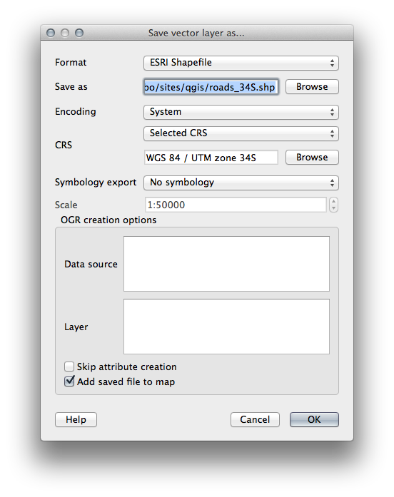
Noul fișier shape va fi creat, iar stratul rezultat va fi adăugat la hartă.

• Eliminați vechiul strat roads.

Repeat this process for each layer, creating a new shapefile and layer with “_34S” appended to the original name and removing each of the old layers.

Once you have completed the process for each layer, right click on any layer and click Zoom to layer extent to focus the map to the area of interest.

Now that we have converted OSM’s data to a UTM projection, we can begin our calculations.

7.2.8. Follow Along: Analyzing the Problem: Distances From Schools and Roads¶

QGIS allows you to calculate distances from any vector object.

• Make sure that only the roads_34S and houses_34S layers are visible, to simplify the map while you’re working.
• Click on the Vector ‣ Geoprocessing Tools ‣ Buffer(s) tool:

This gives you a new dialog.

• Setați-l astfel:

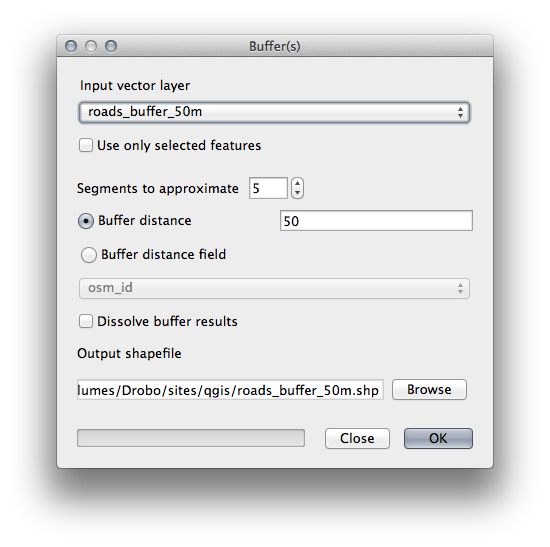
The Buffer distance is in meters because our input dataset is in a Projected Coordinate System that uses meter as its basic measurement unit. This is why we needed to use projected data.

• Save the resulting layer under exercise_data/residential_development/ as roads_buffer_50m.shp.
• Click OK and it will create the buffer.
• When it asks you if it should “add the new layer to the TOC”, click Yes. (“TOC” stands for “Table of Contents”, by which it means the Layers list).
• Close the Buffer(s) dialog.

Now your map will look something like this:

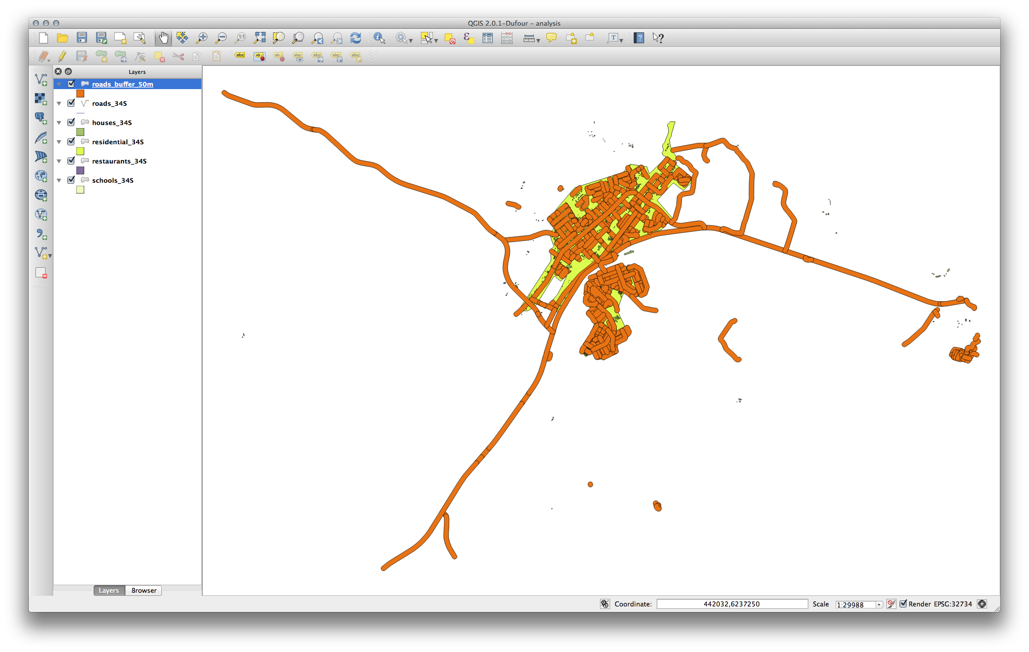
If your new layer is at the top of the Layers list, it will probably obscure much of your map, but this gives us all the areas in your region which are within 50m of a road.

However, you’ll notice that there are distinct areas within our buffer, which correspond to all the individual roads. To get rid of this problem, remove the layer and re-create the buffer using the settings shown here:

• Note that we’re now checking the Dissolve buffer results box.
• Save the output under the same name as before (click Yes when it asks your permission to overwrite the old one).
• Click OK and close the Buffer(s) dialog again.

Once you’ve added the layer to the Layers list, it will look like this:

Now there are no unnecessary subdivisions.

7.2.9. Try Yourself Distance from schools¶

• Use the same approach as above and create a buffer for your schools.

It needs to be 1 km in radius, and saved under the usual directory as schools_buffer_1km.shp.

Check your results

7.2.10. Follow Along: Overlapping Areas¶

Now we have areas where the road is 50 meters away and there’s a school within 1 km (direct line, not by road). But obviously, we only want the areas where both of these criteria are satisfied. To do that, we’ll need to use the Intersect tool. Find it under Vector ‣ Geoprocessing Tools ‣ Intersect. Set it up like this:

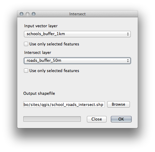
The two input layers are the two buffers; the save location is as usual; and the file name is road_school_buffers_intersect.shp. Once it’s set up like this, click OK and add the layer to the Layers list when prompted.

In the image below, the blue areas show us where both distance criteria are satisfied at once!

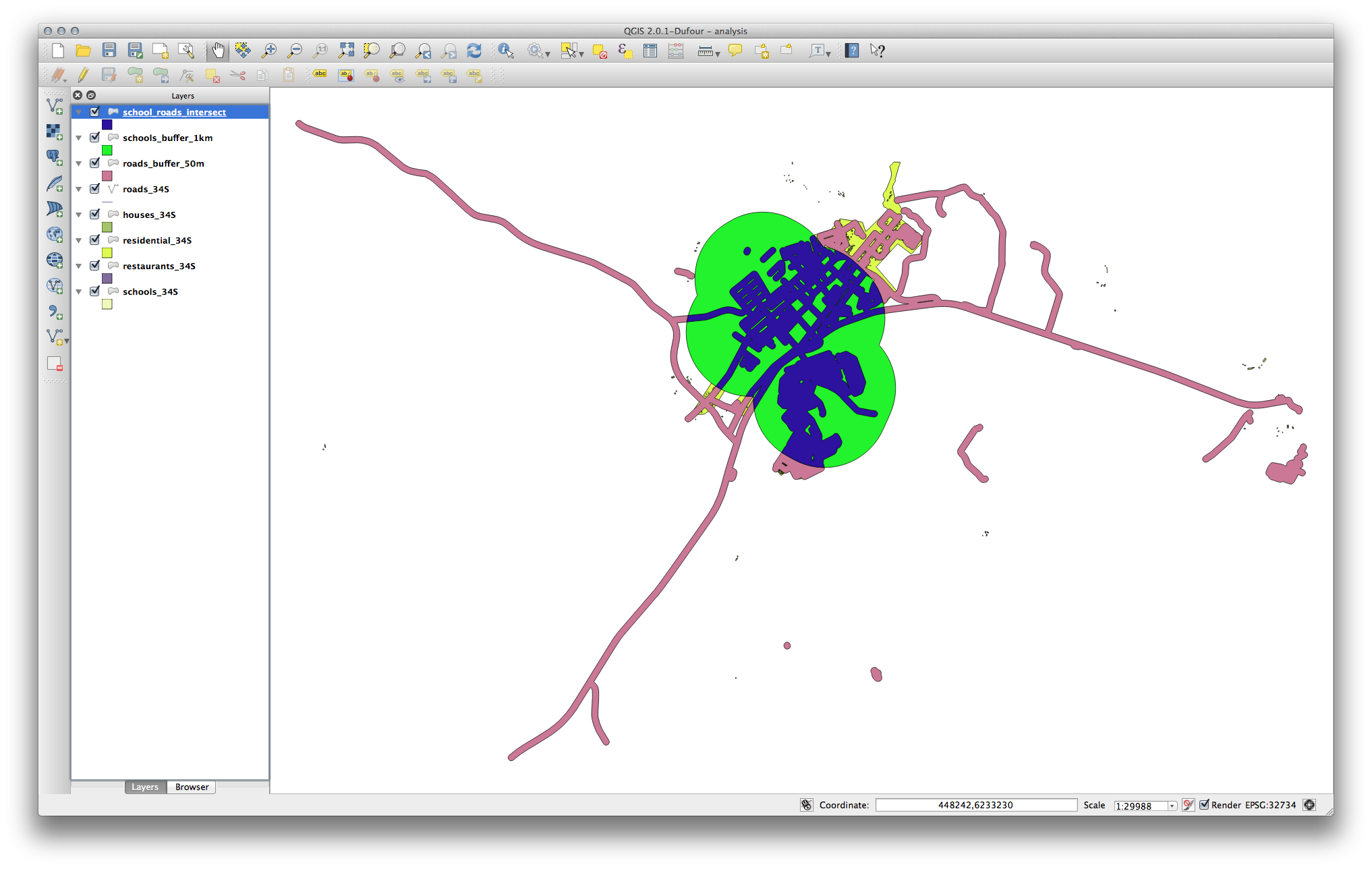
You may remove the two buffer layers and only keep the one that shows where they overlap, since that’s what we really wanted to know in the first place:

7.2.11. Follow Along: Select the Buildings¶

Now you’ve got the area that the buildings must overlap. Next, you want to select the buildings in that area.

• Click on the menu entry Vector ‣ Research Tools ‣ Select by location. A dialog will appear.

• Setați-l astfel:

• Click OK, then Close.
• You’ll probably find that not much seems to have changed. If so, move the school_roads_intersect layer to the bottom of the layers list, then zoom in:

The buildings highlighted in yellow are those which match our criteria and are selected, while the buildings in green are those which do not. We can now save the selected buildings as a new layer.

• Right-click on the houses_34S layer in the Layers list.
• Select Save Selection As....
• Set the dialog up like this:

• The file name is well_located_houses.shp.

• Clic pe OK

Now you have the selection as a separate layer and can remove the houses_34S layer.

7.2.12. Try Yourself Further Filter our Buildings¶

We now have a layer which shows us all the buildings within 1km of a school and within 50m of a road. We now need to reduce that selection to only show buildings which are within 500m of a restaurant.

Using the processes described above, create a new layer called houses_restaurants_500m which further filters your well_located_houses layer to show only those which are within 500m of a restaurant.

Check your results

7.2.13. Follow Along: Select Buildings of the Right Size¶

To see which buildings are the correct size (more than 100 square meters), we first need to calculate their size.

• Open the attribute table for the houses_restaurants_500m layer.
• Enter edit mode and open the field calculator.

• Setați-l astfel:

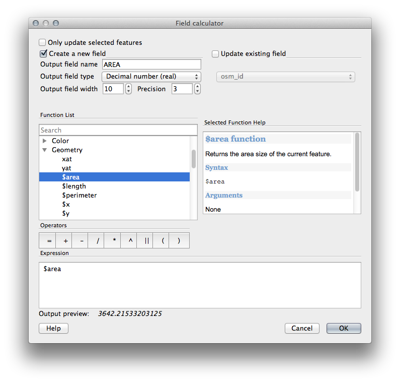
• If you can’t find AREA in the list, try creating a new field as you did in the previous lesson of this module.

• Clic pe OK

• Scroll to the right of the attribute table; your AREA field now has areas in metres for all the buildings in your houses_restaurants_500m layer.
• Click the edit mode button again to finish editing, and save your edits when prompted.
• Build a query as earlier in this lesson:

• Click OK. Your map should now only show you those buildings which match our starting criteria and which are more than 100m squared in size.

7.2.14. Try Yourself¶

• Save your solution as a new layer, using the approach you learned above for doing so. The file should be saved under the usual directory, with the name solution.shp.

7.2.15. In Conclusion¶

Using the GIS problem-solving approach together with QGIS vector analysis tools, you were able to solve a problem with multiple criteria quickly and easily.

7.2.16. What’s Next?¶

In the next lesson, we’ll look at how to calculate the shortest distance along the road from one point to another.